
How to make ice melt faster ? Experiment with two ice cubes.
Last year I volunteered to talk about Arctic and Antarctic in my son’s class who was 5 at the time. I can honestly say that preparing for this 30 minutes session took me longer than for most talks I present at international conferences. Most of my time was taken learning about, and printing, cutting, sticking dozens of Arctic and Antarctic animals (catchy song here) on little cards, but when the dreaded day arrived by far the most successful part of my presentation was a simple experiment involving ice cubes (who needs ipads when kids go bananas for ice cubes ?). I put some ice cubes in an empty glass (figure 1 left) and in a glass half full with water at room temperature (figure 1 right) and asked them to guess which ice cubes will melt faster? If that sounds obvious to you well done you have a great intuitive grasp of thermodynamic concepts, if not you might want to look towards relative heat capacities of water, air and ice and think about heat transfer efficiency REF…but by now you might be wondering where I am going with this.
What about a much bigger ice cube (sea ice) ?
Funnily at the same time we had (with colleagues from CPOM@Reading and from the University of Maryland) just started working on a project using a sea ice model to try and estimate the relative importance of various processes controlling the melt of Arctic sea ice. See the analogy with the ice cubes? After all sea ice is nothing more that a slightly salty, extremely thin ice cube, typically ~1m thick and ~1000km long floating on the Arctic Ocean (a 5cm long ice cube with the same aspect ratio would be 50nm thick!). Like ice cubes sea ice can melt from the top, the bottom and the sides (sea ice can also melt from within due to entrapped pockets of saline water or brine) and like in the example of the ice cubes the same increase of the temperature of the ocean (or water) and atmosphere (air) leads to a much faster melt rate at the ice-water interface. That’s about it for the analogies. Sea ice is in fact a bit more complex and can be found in different states (new ice, young ice, first year ice, multi-year ice, etc), can be more or less deformed, fragmented or porous, is often covered by a layer of snow, and during the melt season by melt ponds at its surface and by under-ice ponds of low salinity water at its bottom. All these characteristics of the ice play a key role in controlling the exchange of heat, salt, moisture (and even momentum) at the interfaces between the atmosphere, the ice and the ocean. Figure 2 illustrates some of the processes at play in this "sea ice orchestra" where according to Alek Petty the “job of the conductor (sea ice modeller) is to ‘tune’ the musicians (parameters) to keep the sound (model) in-key (accurate).”
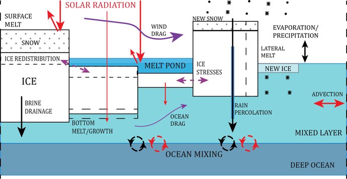 Schematic of the new prognostic ML module and of the other main thermodynamic processes included in the sea ice model CICE. The main heat fluxes are highlighted in red, while the main salt and freshwater fluxes are shown in black. Figure by Alek Petty adapted from [Tsamados et al. 2015].
Results of our model sensitivity study
Finally after more than a year the initial project idea has turned into a paper that will be published today as part of a special issue of the Philosophical Transactions A (the oldest scientific journal) following last year’s Royal Society meeting on the “Arctic sea ice reduction: the evidence, models and impacts”. In this study in addition to the parameterization schemes already implemented in the state of the art Los Alamos community sea ice model CICE, v. 5.0.2 (e.g. explicit melt ponds, a form drag parameterization and a halodynamic brine drainage scheme), we implemented in the model and tested three new schemes: (i) a prognostic ML model; (ii) a three equation boundary condition; and (iii) a parameterization of lateral melting explicitly accounting for the average floe size and floe size distribution dependence. For each simulation, the total melt was decomposed into its surface, bottom and lateral melt components (see figure 3 for our reference run) to assess the relative importance of the processes driving the melt and how this varies regionally and temporally. For most simulations we found bottom melt to be the largest contributor to the total ice melt of Arctic (about two-thirds), surface melt to drive larger inter-annual variability and lateral melt to play an important role in the low concentration ice regions of the marginal ice zones at the ice edge. Overall all parameterizations played a significant role and this sensitivity study highlights the fact that model response uncertainty could dominate overall uncertainty of sea ice characteristics in Global Circulation Models (GCMs). Further work using coupled ice-ocean and fully coupled atmosphere-ice-ocean models is a natural extension of this work. In addition precise validation and calibration of the parameters and physics of the model against observations are needed more than ever if we want to predict more accurately when the “big ice cube” will eventually melt?
Maps of the average July top melt (left), bottom melt (center) and lateral melt (right) over the period 1994 to 2013 for the reference model run of our study. The melt rates are given in cm/day. From [Tsamados et al. 2015].
References